BackPropagation #
\(\)Single-hidden Layer Feedforward Neural Network #
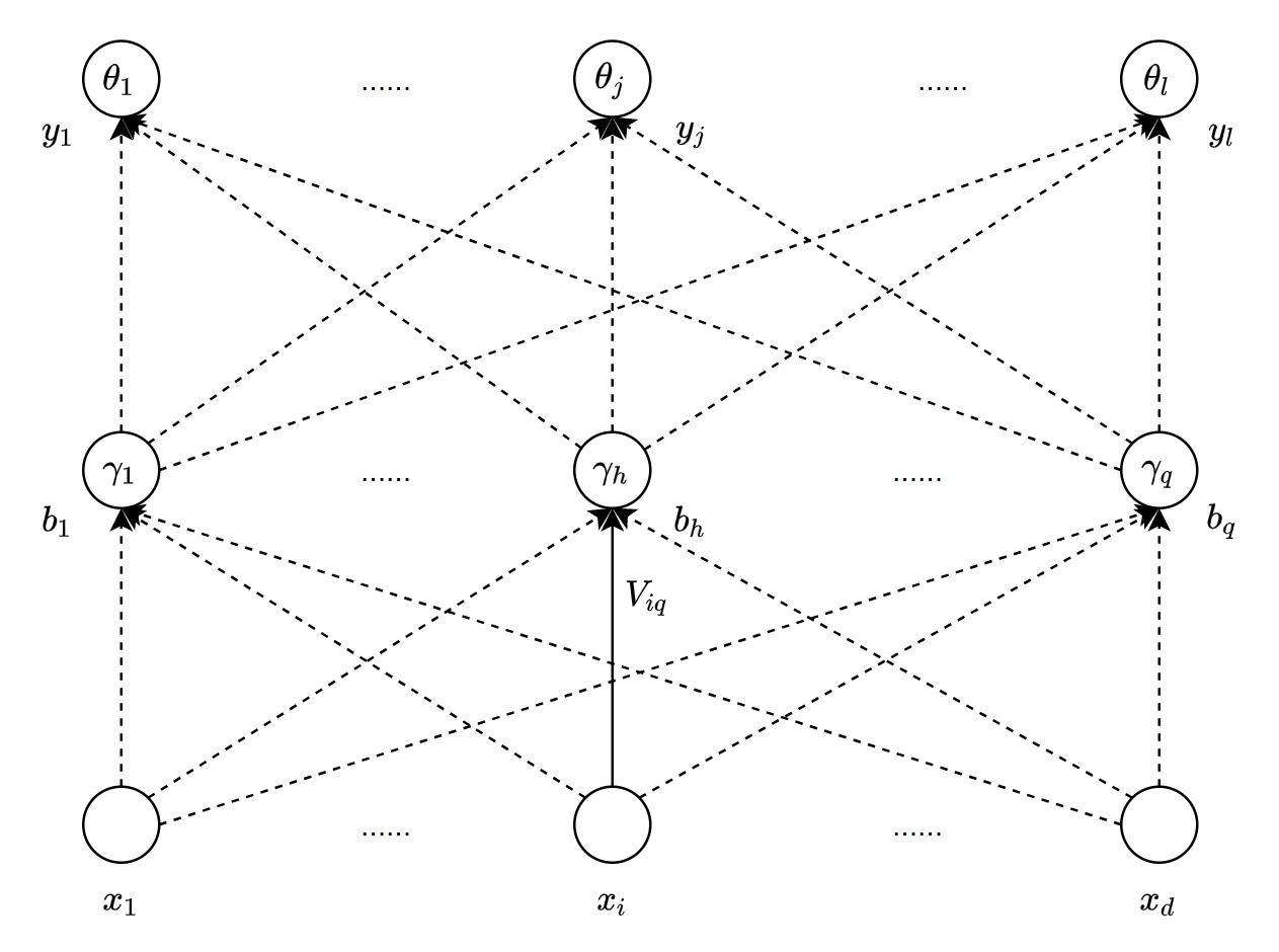
| input | output | |
|---|---|---|
| output layer | $\beta_j=\sum_{h=1}^{q} \omega_{h j} b_{h}$ | $\hat{y}_{j}^{k}=f\left(\beta_j-\theta_j\right)$ |
| hidden layer | $\alpha_h=\sum_{i=1}^{d} v_{i h} x_{i}$ | $b_{n}=f\left(\alpha_{i h}-\gamma_{h}\right)$ |
| input layer | $x_i$ | . |
LossFunction #
累计误差$E_k$,目标$min E_k$
$$ E_{k}=\frac{1}{2} \sum_{j=1}^{l}\left(\hat{y}_{j}^{k}-y_{j}\right)^{2} $$
Iterative Equations1 #
隐层到输出层连接边权值变化
$$ \Delta \omega_{h}=-\eta \frac{\partial E_{k}}{a \omega_{k j}} $$
$$ \begin{aligned} \frac{\partial E_{k}}{\partial \omega_{h j}} &=\frac{\alpha E_{k}}{\partial \hat{y}_{j}^{k}} \cdot \frac{\partial \hat{y}_{j}^{k}}{\partial \beta_{j}} \cdot \frac{\partial \beta_{j}}{\partial \omega_{h j}} \newline &=\left(\hat{y}_{j}^{k}-y_{j}^{k}\right) f^{\prime}\left(\beta_{j}-\theta_{j}\right) \cdot b_{h} \end{aligned} $$
输出层阈值变化
$$ \Delta \theta_{j}=-\eta \frac{\partial E_k}{\partial \theta_{j}} $$
$$ \begin{aligned} \frac{\partial E_k}{\partial \theta_{j}} &=\frac{\partial E_{k}}{\partial \hat{y}_{j}^{k}} \cdot \frac{\partial \hat{y}_{j}^{k}}{\partial \theta_j} \newline &=\left(\hat{y}_{j}^{k}-y_{j}^{k}\right) \cdot f^{\prime}\left(\beta_{i}-\theta_{j}\right) \cdot(-1)=g_{j} \end{aligned} $$
输入层到隐层连接边权值变化
$$ \Delta v_{i h}=-\eta \frac{\partial E k}{\partial V_{i h}} $$
$$ \begin{aligned} \frac{\partial E_k}{\partial v_{i h}}&=\sum_{j=1}^{l} \frac{\alpha E_{k}}{\partial \hat{y}_{j}^{k}} \cdot \frac{\partial \hat{y}_{j}^{k}}{\partial \beta_{j}} \cdot \frac{\partial \beta_{j}}{\partial b_{h}} \cdot \frac{\partial b_{h}}{\partial \alpha_{h}} \cdot \frac{\partial \alpha_{h}}{\partial v_{i h}} \newline &=\sum_{j=1}^{k}\left(\hat{y}_{j}^{k}-y_{5}^{k}\right) \cdot f^{\prime}\left(\beta_{j}-\theta_{j}\right) \cdot \frac{\partial \beta_{j}}{\partial b_{j}} \cdot \frac{\partial b_{h}}{\partial \alpha_{h}} \cdot \frac{\partial \alpha_{h}}{\partial v_{i h}} \newline &=\left[\sum_{j=1}^{l}\left(\hat{y}_{j}^{k}-y_{j}^{k}\right) \cdot f^{\prime}\left(\beta_{j}-\theta_{j}\right) \cdot \omega_{h j}\right] \cdot \frac{\partial b_{h}}{\partial \alpha_{h}} \cdot \frac{\partial \alpha_{h}}{\partial v_{i h}} \end{aligned} $$
通常可以根据经验公式 $m=log_2 ( n )$, ( $m$为隐层节点数,$n$为输入层节点数 ) 得到隐层应节点数。
Examples #
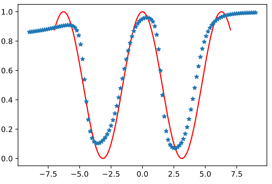
Show an Example: fit $0.5*(cos(x)+1)$
- 测试
max_iter=10000, error=0.0001, same_error_times=10iterated 10000/10000 times, error 0.2785599852590231.
Show an Example: fit $0.5*cos(x_1)*sin(x_2)$
import numpy as np
import pandas as pd
import matplotlib.pyplot as plt
# 二维训练集样本
x = np.array((np.linspace(-7, 7, 200), np.linspace(-7, 7, 200))).T
y = np.expand_dims((np.cos(x[:, 0]) + np.sin(x[:, 1])) * 0.5, 1)
bp = BackPropagation(q=3, lr_1=0.5, lr_2=0.6)
bp.fit(x, y, max_iter=1000, error=0.0001, same_error_times=10)
iterated 1000/1000 times, error is 19.441564975483463, covergent 1 times.
ax = plt.subplot(111, projection="3d")
ax.plot3D(x[:, 0], x[:, 1], y[:, 0], c="w")
ax.plot3D(x_test[:, 0], x_test[:, 1], Y_Y[:, 0], c="b")
[<mpl_toolkits.mplot3d.art3d.Line3D at 0x7fb286c26340>]

# 二维训练集样本
x = np.array((np.linspace(-7, 7, 200), np.linspace(-7, 7, 200))).T
y = np.expand_dims((np.cos(x[:, 0]) + np.sin(x[:, 1])) * 0.5, 1)
bp = BackPropagation(q=5, lr_1=0.8, lr_2=0.6)
bp.fit(x, y, max_iter=1000, error=0.0001, same_error_times=10)
iterated 568/1000 times, error is 14.466125682677891, covergent 9 times.
# 二维测试集样本
x_test = np.array((np.linspace(-9, 9, 200), np.linspace(-9, 9, 200))).T
Y_Y = bp.predict(x_test)
ax = plt.subplot(111, projection="3d")
ax.plot3D(x[:, 0], x[:, 1], y[:, 0], c="w")
ax.plot3D(x_test[:, 0], x_test[:, 1], Y_Y[:, 0], c="b")
[<mpl_toolkits.mplot3d.art3d.Line3D at 0x7fb286b2af70>]

start_time = time.time()
bp.fit(
    x,
    y,
    max_iter=1000000,
    error=0.00001,
    same_error_times=200,
    Rh=bp.Rh,
    Thej=bp.Thej,
    Vih=bp.Vih,
    Whj=bp.Whj,
)
end_time = time.time()
print("training costs {} s".format(end_time - start_time))
iterated 21841/1000000 times, error is 13.866926271017798, covergent 199 times.
training costs 573.6911239624023 s
# 二维测试集样本
x_test = np.array((np.linspace(-9, 9, 200), np.linspace(-9, 9, 200))).T
Y_Y = bp.predict(x_test)
ax = plt.subplot(111, projection="3d")
ax.plot3D(x[:, 0], x[:, 1], y[:, 0], c="w")
ax.plot3D(x_test[:, 0], x_test[:, 1], Y_Y[:, 0], c="b")
[<mpl_toolkits.mplot3d.art3d.Line3D at 0x7fb28699fcd0>]

Code #
Show Code
#%%
import numpy as np
import pandas as pd
import matplotlib.pyplot as plt

# %%
path = "/home/ias/workdir/ml-primary/ml-notes/data/watermelon_data3.0.csv"
data = pd.read_csv(path)
data.head()

# %%
from sklearn import preprocessing

enc = preprocessing.OneHotEncoder()
a = np.array(enc.fit_transform(data.iloc[:, :7]).toarray())
b = np.array(data.iloc[:, 7:9])
X = np.c_[a, b]
y = np.array(enc.fit_transform(data.iloc[:, 9:]).toarray())

#%%
class BackPropagation:
    def __init__(self, q=1, lr_1=0.1, lr_2=0.1) -> None:
        self.q = q
        self.lr_1 = lr_1
        self.lr_2 = lr_2

    def sigmoid(self, v, the):
        return 1 / (1 + np.exp(-(v - the)))

    def fit(
        self,
        X,
        Y,
        max_iter=50,
        error=0.001,
        same_error_times=5,
        Rh=None,
        Thej=None,
        Vih=None,
        Whj=None,
    ):
        """fit AI is creating summary for fit

        Args:
            X ([type]): [N * d]
            Y ([type]): [N * m]
            max_iter (int, optional): [description]. Defaults to 50.
        """
        # init
        N, d = np.shape(X)
        m = np.shape(Y)[1]
        Rh = np.random.random(self.q) if Rh is None else Rh
        Thej = np.random.random(m) if Thej is None else Thej
        Vih = np.random.random((d, self.q)) if Vih is None else Vih
        Whj = np.random.random((self.q, m)) if Whj is None else Whj

        error_list = []
        old_Ek = 0
        cur = 0
        sn = 0
        while cur < max_iter:
            Ek = np.zeros(N)
            for k in range(N):
                # calculate Bh
                Ah = np.zeros(self.q)
                Bh = np.zeros(self.q)
                for h in range(self.q):
                    Ah[h] = np.dot(X[k], Vih[:, h])
                    Bh[h] = self.sigmoid(Ah[h], Rh[h])
                # calculate Yj
                Pj = np.zeros(m)
                Yj = np.zeros(m)
                Gj = np.zeros(m)
                for j in range(m):
                    Pj[j] = np.dot(Bh, Whj[:, j])
                    Yj[j] = self.sigmoid(Pj[j], Thej[j])
                    # calculate Gj
                    Gj[j] = Yj[j] * (1 - Yj[j]) * (Y[k][j] - Yj[j])
                # calculate Eh
                Eh = np.zeros(self.q)
                for h in range(self.q):
                    Eh[h] = Bh[h] * (1 - Bh[h]) * np.dot(Gj, Whj[h, :])
                # update
                Whj += self.lr_1 * np.reshape(np.kron(Bh, Gj), (self.q, m))
                Vih += self.lr_2 * np.reshape(np.kron(X[k], Eh), (d, self.q))
                Thej += -self.lr_1 * Gj
                Rh += -self.lr_2 * Eh
                # calculate Ek
                Ek[k] = 0.5 * np.sum(np.power(Yj - Y[k], 2))
            if abs(old_Ek - sum(Ek)) < error:
                sn += 1
                if sn >= same_error_times:
                    break
            else:
                old_Ek = sum(Ek)
                error_list.append(old_Ek)
                sn = 0
            cur += 1
            print(
                "\riterated {}/{} times, error is {}, covergent {} times.".format(
                    cur, max_iter, old_Ek, sn
                ),
                end="",
            )
        print("", end="\n")
        print(
            "\r Finished, iterated {}/{} times, error is {}, covergent {} times.".format(
                cur, max_iter, old_Ek, sn
            ),
            end="",
        )
        self.Rh = Rh
        self.Thej = Thej
        self.Vih = Vih
        self.Whj = Whj
        self.error_list = error_list

    def predict(self, x_test):
        Y_Y = np.zeros((np.shape(x_test)[0], np.shape(self.Whj)[1]))
        for i in range(len(x_test)):
            A_H = np.dot(x_test[i], self.Vih)
            B_V = np.array(
                [self.sigmoid(A_H[h], self.Rh[h]) for h in range(len(A_H))]
            )
            P_J = np.dot(B_V, self.Whj)
            Y_O = np.array(
                [self.sigmoid(P_J[j], self.Thej[j]) for j in range(len(P_J))]
            )
            Y_Y[i] = Y_O
        return Y_Y


# %%
# 训练集样本
x = np.array([np.linspace(-7, 7, 200)]).T
y = (np.cos(x) + 1) / 2
bp = BackPropagation(q=3, lr_1=0.3)
bp.fit(x, y, max_iter=1000, error=0.0001, same_error_times=10)

# %%
# 测试集样本
x_test = np.array([np.linspace(-9, 9, 120)]).T
# 测试集结果
# y_predict = network.feedforward(x_test)
Y_Y = np.zeros(len(x_test))
for i in range(len(x_test)):
    A_H = x_test[i] * bp.Vih
    B_V = [bp.sigmoid(v, bp.Rh) for v in A_H]
    Y_M = np.shape(bp.Whj)[1]
    Y_J = np.zeros(Y_M)
    Y_O = np.zeros(Y_M)
    for j in range(Y_M):
        Y_J[j] = np.dot(B_V, bp.Whj[:, j])
        Y_O[j] = bp.sigmoid(Y_J[j], bp.Thej[j])
    Y_Y[i] = Y_O

# %%
nbp = BackPropagation(q=3, lr_1=0.3)
nbp.fit(
    x,
    y,
    max_iter=1000,
    error=0.0001,
    same_error_times=10,
    Rh=bp.Rh,
    Thej=bp.Thej,
    Vih=bp.Vih,
    Whj=bp.Whj,
)
x_test = np.array([np.linspace(-9, 9, 120)]).T
Y_Y = nbp.predict(x_test)

plt.plot(x, y, "r", x_test, Y_Y, "*")
# %%
# 二维训练集样本
import time

start_time = time.time()

x = np.array((np.linspace(-7, 7, 200), np.linspace(-7, 7, 200))).T
y = np.expand_dims((np.cos(x[:, 0]) + np.sin(x[:, 1])) * 0.5, 1)
bp = BackPropagation(q=5, lr_1=0.8, lr_2=0.4)
bp.fit(x, y, max_iter=1000000, error=0.0001, same_error_times=100)

end_time = time.time()
print("training costs {} s".format(end_time - start_time))

# %%
# 二维测试集样本
x_test = np.array((np.linspace(-9, 9, 200), np.linspace(-9, 9, 200))).T
Y_Y = bp.predict(x_test)

# %%
ax = plt.subplot(111, projection="3d")
ax.plot3D(x[:, 0], x[:, 1], y[:, 0], c="w")
ax.plot3D(x_test[:, 0], x_test[:, 1], Y_Y[:, 0], c="b")


# %%
start_time = time.time()
nbp = BackPropagation(q=5, lr_1=0.3, lr_2=0.1)
nbp.fit(
    x,
    y,
    max_iter=1000000,
    error=0.00001,
    same_error_times=200,
    Rh=bp.Rh,
    Thej=bp.Thej,
    Vih=bp.Vih,
    Whj=bp.Whj,
)
end_time = time.time()
print("training costs {} s".format(end_time - start_time))

# %%